MaxDiff Sample Size: 200 Per Subgroup, Then Check the Power

How many respondents do you need for MaxDiff research? Explore sample size recommendations, statistical power, subgroup analysis and study design.

Andy Booth

Managing Consultant

Aim for at least 200 respondents per reportable subgroup, or around 300 overall, for a MaxDiff study to deliver stable aggregate results. That baseline typically rises when you introduce hierarchical Bayes (HB) modelling, latent class segmentation, or several subgroups you plan to report separately. For a figure you can defend to stakeholders rather than one borrowed from habit, a short confidence-and-power calculation offers a systematic approach.

For hierarchical Bayes, latent class, or individual preference analysis, plan for 300 to 500 respondents or more; separate subgroup reporting raises the total further.
With a 0.16 standard error and a 0.223 detectable difference, Sawtooth’s example needs 227 respondents for 95% confidence, or 1,600 with 80% power.
Show four to five items per task, keep questionnaires to about 25 questions, and display each item at least three times per respondent.
If budgets limit sample size, pool closely related subgroups, shorten the item list, or field sequential waves rather than underpowering a single wave.
Samples below 100 respondents can indicate likely winners and losers, but rankings may shift on rerun and subgroup comparisons remain unreliable.

Recommended sample ranges and when to use each

MaxDiff sample size is not a single number, it is a decision that depends on what you need the data to do. At the lower end, samples under 100 respondents will give you a directional sense of which items win and lose, but the rankings will shift if you rerun the study, and subgroup cuts become unreliable. A common baseline for many commercial projects sits higher than that.

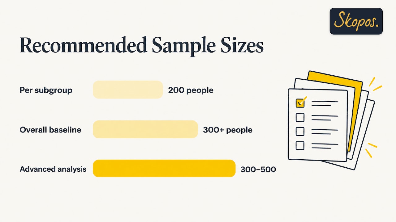
Common practice, reflected in guidance from Bentley University’s user experience centre, is to treat 200 respondents per subgroup, or 300 or more overall, as the threshold for reliable aggregate-level results. That range works well when you are ranking features, messages or concepts at the total-sample level and do not need to model individual preferences.

Three situations typically push the target higher:

You plan to run HB or latent class modelling, which estimates preferences at the individual or segment level rather than pooling everyone together.
You have more than 12 to 15 items in your list, which spreads respondent attention thinner across the design.
You need several subgroups reported independently, each of which needs its own 200-respondent base.

In those cases, planning for 300 to 500 respondents, sometimes more, avoids a rerun. The trade-off is straightforward: every extra respondent costs money and fielding time, and because statistical precision improves with the square root of sample size rather than in a straight line, the gains from pushing past your required threshold shrink quickly. Doubling your sample does not double your precision, so there is little value in over-building once you have hit the range your analysis plan actually needs.

How to calculate sample size: confidence, power and a worked example

Rules of thumb are useful for a first estimate, but when a client or stakeholder asks why you chose a particular number, a calculation is more persuasive than a convention. The method used by Sawtooth Software’s sample-size guidance scales a known standard error (SE) to a target sample using a simple rule: target detectable difference equals observed detectable difference multiplied by the square root of 400 divided by n. The constant 400 appears because Sawtooth’s worked examples typically estimate the observed SE from a 400-respondent pilot or simulation in Lighthouse Studio.

Statistic: Increasing a MaxDiff sample from 400 to 4,000 respondents reduces the detectable utility difference from roughly 0.168 to roughly 0.053 in Sawtooth’s worked examples, illustrating how much larger a sample has to grow for comparatively modest gains in precision.

A practical calculation runs in four steps:

Estimate your observed standard error from a pilot sample or a simulated dataset, since this figure is specific to your items and design rather than universal.
Decide the smallest utility difference you need to detect reliably. A commonly used benchmark is ln(1.25), which equals 0.223, representing a 25% relative preference difference.
Combine Z-values for your confidence and power targets. For 95% confidence alone, use 1.96; to also achieve 80% power, add 0.84, giving a combined value of 2.80.
Solve for n by rearranging the scaling formula around your target detectable difference and combined Z-value.

Sawtooth’s worked example detecting a 0.223 utility difference with an observed SE of 0.16 produces roughly 227 respondents when confidence alone is the target, rising to roughly 1,600 when the design must also achieve 80% power. If your pilot SE comes out higher or lower than 0.16, rerun the same formula with your own figure rather than reusing someone else’s worked numbers.

Design constraints that change required n

Sample size never works in isolation from the design choices sitting around it. Items per set, the number of questions you ask, and how often each item appears all change how much data you extract from each respondent, which in turn changes how large your sample needs to be.

Showing four to five items per question is the pragmatic balance supported by empirical studies on task length and items per set: fewer items force sharper trade-offs, while more items slow respondents down without improving predictive validity.
Keep total MaxDiff questions to roughly 25 or fewer to limit fatigue, favouring more short questions over fewer long ones for the same respondent time budget.
Aim to show each item at least three times per respondent, a threshold Sawtooth's MaxDiff calculator guidance treats as the practical floor for stable item-level utilities.
Where the study spans multiple markets, keep the design and item wording comparable across them so sample-size decisions are not undermined by inconsistent task structures; our guidance on multi-market comparability covers this in more detail.

Pro Tip: Track median task completion time and early dropout during soft launch, not after full fielding, so you can adjust item count or question length before the bulk of your sample comes in.

Advanced analyses and subgroup reporting

Aggregate results and individual-level models ask very different things of your sample. A simple total-sample ranking pools every respondent’s choices together, which is why 300 respondents can be enough for that purpose. HB and latent class models work differently: they estimate a distribution of preferences across the sample or across inferred segments, which needs more data per estimated parameter to converge reliably.

Plan for 300 to 500 respondents or more whenever your analysis plan includes HB estimation, latent class segmentation, or any individual-level inference.
Apply the same 200-respondent-per-subgroup rule from the Bentley guidance to each group you intend to report on its own, whether that is by age band, customer tier or region.
Where budget or field access genuinely constrains numbers, consider pooling closely related subgroups, trimming the item list to the questions that matter most, or fielding in sequential waves rather than cutting corners on a single wave's base size.

A simulation study on utility stability found that utility estimates and confidence intervals tend to stabilise well before the full planned sample is reached, and that efficient designs can lower the sample needed to hit a given precision target. That is a reason to check stability during fielding, not a licence to plan a smaller sample from the outset.

Practical checklist for planning a MaxDiff sample

A sample-size decision holds up better when it is documented, not just chosen. Before fielding, work through this sequence:

Write down the decision the research needs to support and the smallest utility difference that would change that decision.
Set a baseline n and, separately, a target for each subgroup you plan to report, noting the tolerance you are willing to accept.
Fix items per set, total questions and a target of at least three appearances per item per respondent.
Run a pilot or simulation to estimate your SE, then scale your final n using the square root of 400 divided by n rule.
Build in fielding QA: dropout thresholds, task time flags and attention checks, covered in more depth in our data quality guidance.

Pro Tip: Paste the baseline n, subgroup targets and item-appearance rule straight into your SOW before fielding starts, so changes to scope are visible and costed rather than discovered halfway through analysis.

Sample size is rarely treated as a single lookup. A short pilot or simulation is often run to estimate the real standard error for the item list, then the rule-of-thumb ranges are weighed against budget and the subgroups that actually need reporting. Item stability and fielding quality checks accompany the headline number, because a sample that hits its target n but fails on dropout or task time has not solved the problem.

‍

How Skopos can help with MaxDiff design and sample planning

Getting MaxDiff sample size right is one part of a design that also has to work for respondents, for the analysis plan, and for the budget you are given to field it. We handle MaxDiff and conjoint design, power analysis, HB and latent class modelling, and the fielding and quality checks that keep a sample usable once it is in.

A typical engagement starts with a short pilot to estimate your standard error, moves into a simulation to confirm the sample plan, then runs fielding with the dropout and task-time monitoring built in from the checklist above, finishing with an executive-ready debrief rather than a raw data file. If MaxDiff sits within a wider segmentation or concept-testing programme, our customer segmentation and concept and product testing services pick up where the MaxDiff output leaves off. Visit our insight partner plans to see how Foundation, Growth and Strategic support ongoing research programmes, or get in touch to talk through a specific MaxDiff brief.

FAQ

What is a MaxDiff study?

A MaxDiff (maximum difference) study asks respondents to pick the best and worst items from small sets shown repeatedly, producing a ranked list of preferences across a larger item set. It avoids the scale-use bias common in rating scales, because respondents are forced to trade items off against each other rather than rating everything similarly, as noted in the MetricGate MaxDiff primer.

How do you interpret MaxDiff results?

MaxDiff results are usually reported as rescaled utility scores or probabilities that sum to 100% across items, letting you rank items by relative preference rather than by absolute rating. A difference between two items only matters if it exceeds the detectable difference your sample size supports, which is why the power analysis approach matters alongside the ranking itself.

What is a MaxDiff question?

A MaxDiff question, or task, shows respondents a small subset of items, typically four to five, and asks them to choose the best and the worst from that set. Each respondent answers several of these tasks in sequence, with the design rotating item combinations so every item appears multiple times across the questionnaire.

What is MaxDiff analysis in market research?

MaxDiff analysis in market research is a technique for prioritising features, messages, claims or concepts by forcing respondents into repeated trade-off choices rather than independent ratings. It is widely used for feature prioritisation and claims testing, and the underlying choice data can feed aggregate rankings, HB models or segmentation work depending on the sample size and analysis plan.